Model and Analysis of Duct Placement Factor in Fiber Optic Cable Pulling – The effect of COF on the Duct Displacement Model
In this article, we show how the Coefficient of Friction (COF) impacts the cable tension when it is pulled through duct undulations or regular displacements.
Reel-memory displacement in continuous fiber optic duct has been modeled as shown in Figure 1. Duct displacement is treated as a “repeating wave” running the length of the conduit, with an “amplitude (A)” and a “period (P)”. Part 1 of this series describes the theory behind this model. Part 2 of this series shows how we can calculate the angle introduced (per unit of length) by the regular displacements. Then, the pulling equations can be used to estimate pulling tension based on the total angle in a pull. In this installment, Part 3 shows how the Coefficient of Friction (COF) impacts the cable tension when it is pulled through these duct undulations or regular displacements.
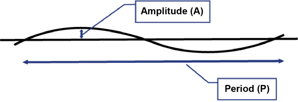
FIGURE 1. Model of Regular Duct Displacement
Previous posts have shown the effect of amplitude and period variations on bend angle and pulling tension. The analysis shows that, to make long fiber pulls (thousands of feet) at safe pulling tensions, the displacement bend must be kept well under 0.5 degrees per foot (1.6 degrees per meter).
| Related Content: Model and Analysis of Duct Displacement Factor in Fiber Optic Cable Pulling-Part 1 |
The Effect of Friction in the Model
We know that friction, measured as the “Coefficient of Friction” (COF), is an important variable in pulling tension. In a straight section of conduit, pulling tension is directly proportional to COF. So, if we double the COF, we double the tension in a pull. Conversely, if we halve the COF, we can pull twice as far with the same tension.
What about friction changes in the continuous displacement approach of this model?
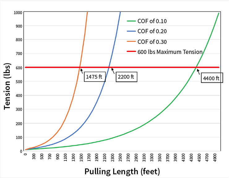
FIGURE 2. Tension vs Pull Length (Displacement Angle = 0.5°/ft)
Figure 2 graphs tension versus distance for a fiber optic pull. The displacement angle was set to 0.5 degrees per foot (1.6 degrees per meter). The calculations use a cable weight of 0.1 lb./ft. (150 gm/m) and an initial incoming tension of 10 lbs. (45 N). Three friction coefficients are calculated (COF = 0.10, COF = 0.20, and COF = 0.30), representing a typical friction range based on both field and laboratory measurements.
The graph shows the importance of minimizing friction. You can pull three times farther with the same tension when the COF is reduced by a factor of three. The distance a cable can be pulled with a given tension is inversely proportional to the friction coefficient, just as in a straight section calculation. The graph estimates 600 lbs. of tension at 4400 feet, 2200 feet, and 14 feet with the friction coefficients of 0.10, 0.20, and 0.30, respectively.
| Related Content: How to Avoid Crushing Fiber Cable During Installation |
The Theory
This linearity is slightly surprising when we look at the simplified form (an approximation*) of the bend pulling equation (Equation 1). The friction is in an exponent, which would not typically imply linearity.
Conduit Bend Tout = Tin eμϴ
Where:
Tout = Tension Out
Tin = Tension in
μ = Coefficient of Friction
ϴ = Angle of Bend (radians)
e = Naperian Log Base
However, on closer examination, we see when “Tension Out” and “Tension In” are constants, the eμϴ factor must also stay constant. Changes in μ (COF) must be offset with reciprocal changes in ϴ. In other words, higher bend angles can be offset by a lower COF.
But ϴ is the total bend angle, which we can describe as:
ϴ = φ * d (Equation 2)
Where:
ϴ = Total Bend Angle
φ = Displacement Angle per Length (0.5 degrees/ft in Figure 2)
d = Pulling Distance or Total Length.
So, if we double μ, the distance must be cut in half to reduce the total angle by the factor of 2. The inverse proportionality results from the total bend building proportionately to the distance in the model.
Previous posts showed that the duct displacement angle can vary by an order of magnitude based on duct placement method (from 0.2° to 2.0°). Equation 1 reinforces the importance of minimizing the displacement angle. It is simply not possible to offset the effect of higher displacements with reduced friction.
| Related Content: The Origins of Lubrication in Cable Blowing: An Interview with Expert Willem Griffioen |
Incoming Tension
Finally, Equation 1 shows the importance of minimum incoming tension. If incoming tension doubles, we see that tension doubles. Pulling distance at a set tension is also reduced significantly.
Calculator Available
If you are interested in getting the calculator (Excel) used in this analysis, please complete the “Email Us” form below. One of our technical people will send you the calculator and contact you to explain data input detail.
*The approximation in Equation 1 is quite accurate when incoming tensions are much greater than the weight of the cable in the bend. However, for the large radius bends predicted by the displacement model, the full equation (which includes a weight component) was used for the graph calculations. Those equations predict a higher tension than the approximation, especially as incoming tension approaches zero.